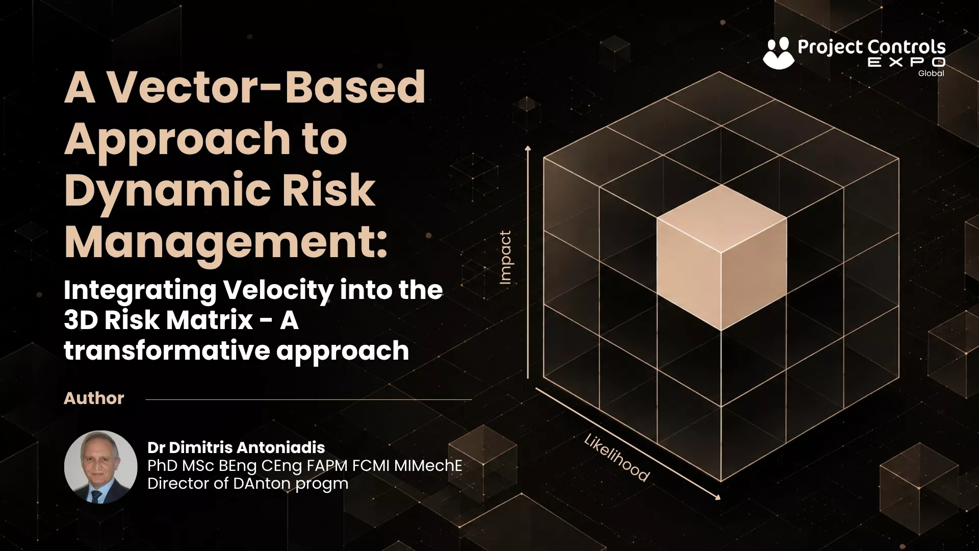
Melbourne Cricket Ground
23-24 November 2026
In this article, the author introduces a transformative approach to risk management by integrating temporal dynamics into the established three-dimensional (3D) risk matrix. Traditional two-dimensional (2D) models, which assess risks based on likelihood and impact, fail to capture the complexity and urgency inherent in modern projects.
Building on the 3D Risk Matrix, where risks are positioned within a cube defined by likelihood, impact on time, and impact on cost, the proposed approach reconceptualises risks as dynamic vectors rather than static points. This shift enables the incorporation of Risk Velocity, a critical and unexplored dimension that measures the speed at which risks materialise and escalate. The author expands on two distinct components of risk velocity, defined as Lead Time Velocity (LTV), representing the approach of a risk toward occurrence, and Impact Time Velocity (ITV), describing the rate at which consequences intensify post-occurrence.
By applying vector mathematics, the proposed approach captures both magnitude and direction, offering a richer representation of risk severity and trajectory. The framework introduces predictive capabilities through vector equations, allowing risk escalation to be modelled as a function of time. This dynamic perspective enhances prioritisation, enabling managers to distinguish between high-impact, slow-moving threats and lower-impact, fast-moving risks that demand immediate action. The author concludes by outlining future directions, including software integration for real-time visualisation and extending the model to additional risk dimensions. The vector-based approach advances risk management from a reactive process to a more proactive one and provides project teams and risk practitioners with much improved foresight and strategic control.
Keywords: Risk Velocity, Risk Management, Vectorisation of Risk, Risk Lead Time Velocity, Risk Impact Time Velocity.
1 How to cite this paper: Antoniadis, D. N. (2026). A Vector-Based Approach to Dynamic Risk Management: Integrating Velocity into the 3D Risk Matrix - A transformative approach; PM World Journal, Vol. XV, Issue II, February. www.pmworldlibrary.net
2026 Dimitris N. Antoniadis
Page 1 of 24
In an era characterised by increasing project complexity and interdependence, the demand for more improved and dynamic risk management methodologies has never been greater. Traditional approaches, while foundational, often fall short in capturing the full, multi-dimensional nature of modern risks. This paper builds upon established risk theory to propose a novel, vector-based framework that integrates the critical dimension of time. By reconceptualising risks as dynamic vectors rather than static points, we can achieve a more nuanced understanding of not only their potential impact but also the speed at which they approach and escalate.
The core practice of risk management is rooted in understanding and addressing uncertainty. The Association for Project Management (APM) Body of Knowledge (2019) provides a concise and powerful definition of risk: "The potential of an action or event to impact the achievement of objectives."
The fundamental purpose of risk management is to proactively assess and manage this uncertainty before potential events materialise. It is a systematic process designed to optimise success by minimising threats and maximising opportunities. By predicting what might deviate from the plan, project leaders can implement actions and responses to reduce uncertainty to an acceptable level, if not minimised completely.
The traditional risk management process operates as a dynamic, cyclical flow, ensuring that risk analysis remains current as new knowledge emerges. This process involves several key stages (APM, 2019):
At the heart of this process lies a fundamental dichotomy in how risks are managed. This separation of concerns is crucial for targeted and effective risk response:
While this structured approach has served projects well, its reliance on conventional, two-dimensional assessment tools presents significant limitations. These tools often struggle to represent the combined impacts of cost and time or to capture the urgency of a threat. It is this gap that the author attempts to address in order to move towards a more robust, three-dimensional framework capable of modelling risk with greater fidelity, supported by mathematical concepts.
Accuracy in visualising and assessing complex risks is a supporting and valuable mechanism for any project team. However, conventional two-dimensional (2D) methodologies have faced growing criticism for their inability to capture the multifaceted nature of modern project threats. In this section the author critiques these shortcomings and introduces the 3D Risk Matrix as a significant advancement, providing a more comprehensive spatial understanding of risk.
The primary concerns with traditional 2D risk methodologies are numerous, leading to subjective outcomes and a lack of confidence in the process among workshop participants and stakeholders. Key criticisms include:
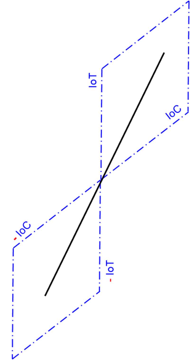
To overcome these issues, the 3D Risk Matrix was developed (Antoniadis & Thorpe, 2003). The proposed model expanded the traditional framework by positioning risks within a three-dimensional space defined by three basic axes:
This approach transforms a risk assessment from a simple product of two variables into a coordinate point within a 3D cube. This allows for a more granular and simultaneous consideration of likelihood, impact on time and impact on cost, as shown below in Figure 1.
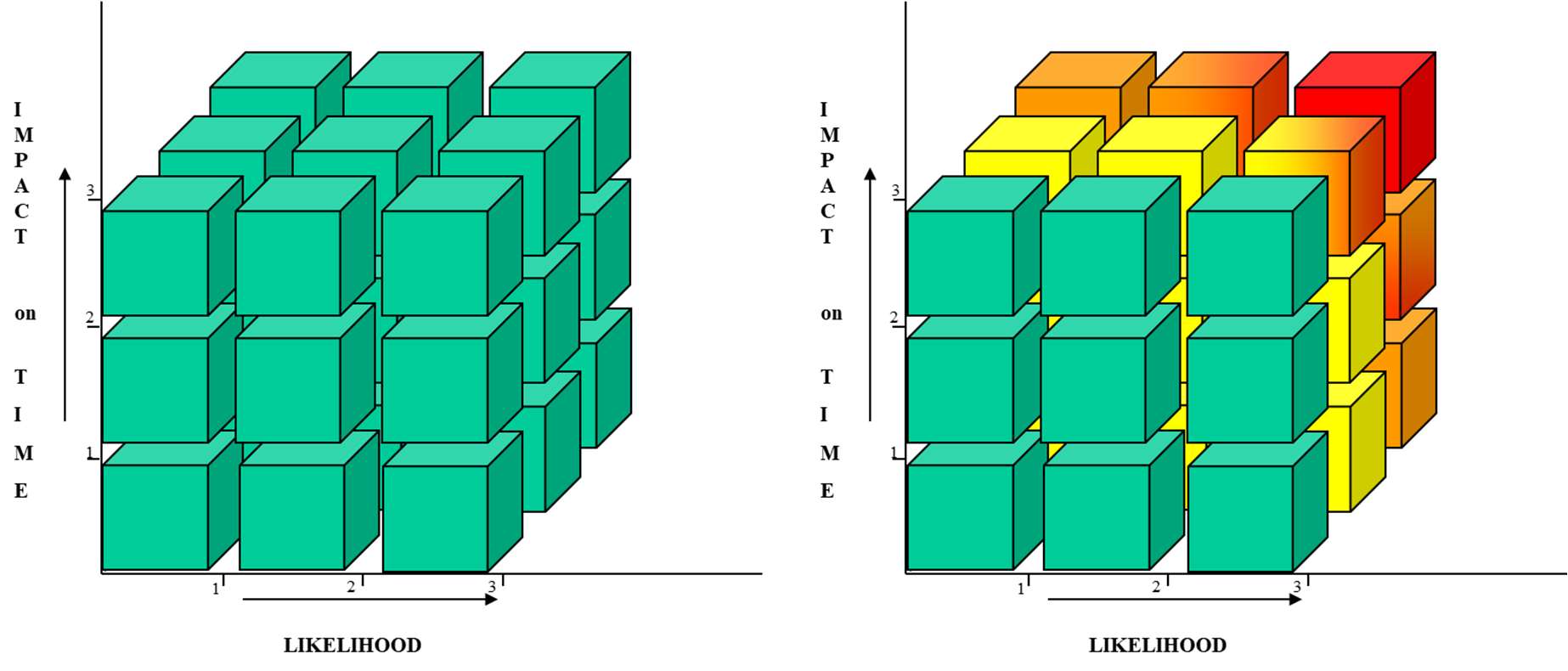
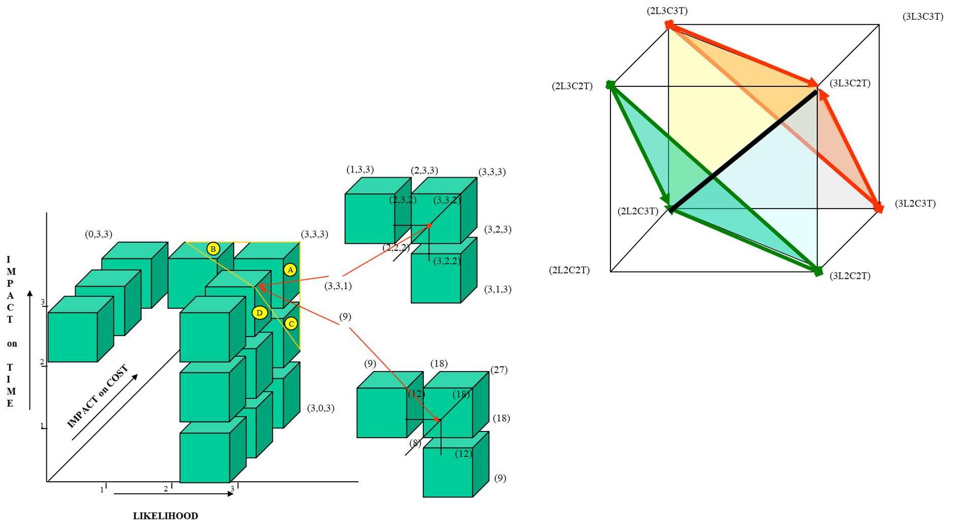
As described in Antoniadis & Thorpe (2003), a core innovation of this methodology is the concept of "Risk Pyramids." Rather than treating risks as isolated points, the model recognises that they can exist in the space between the integer coordinates. Pyramids are formed by connecting adjacent coordinates within the main cube, creating discrete zones of risk priority. This geometric solution allows for the use of decimal values, providing a more nuanced prioritisation. The breakthrough lies in establishing that position, not just magnitude, dictates priority (see Figure 2).
For example, a risk assessed at L=2.5, IoC=2.8, IoT=1.8 yields a product of 12.6 (Antoniadis & Thorpe, 2003). In a 2D system, this might be deprioritised against another risk with a higher product. However, its coordinates place it squarely within a high-priority pyramid, correctly identifying its severity in a way that simple multiplication cannot. Figure 2 below presents, in a 3 x 3 matrix, how the individual blocks are identified and then how these are separated into pyramids. A more detailed description and analysis of this can be found in Antoniadis & Thorpe (2003).
The primary advantages of this methodology (Antoniadis & Thorpe, 2003) are twofold: a profound enhancement in visualisation and a significant increase in analytical granularity. By enabling participants to visualise risks in a 3D landscape, the model improves communication and stakeholder buy-in. Quantitatively, it improves the process of identifying major risks by focusing attention on specific high-priority pyramids, thereby accelerating the workshop process and allowing for more focused mitigation planning. The location within a pyramid provides a more accurate indicator of severity than a simple product score, moving the practice from a qualitative art toward a more quantitative science.
At the ISEC-02 Conference in 2003, the author presented a case study, see Figure 3 below, of applying the 3D Risk Matrix (3DRM) methodology on an airport Fuel Management Unit. Having conducted a workshop to identify the risks using the two methodologies, the author demonstrated that with the 3DRM approach, amber risks should have had a higher risk level(s). Figure 3 below also demonstrates how a number of 'red' risks should have been 'amber' and at least two 'amber risks should have been 'red'.

While the 3D matrix provides a vastly superior spatial understanding of risk, it still treats each threat as a static, fixed point in that space. This perspective, though an improvement, overlooks a critical variable: the speed at which a risk can manifest and cause harm. This sets the stage for the next step(s) in risk theory - the integration of time as a dynamic element.
To manage risk proactively, it is not adequate to understand if a risk might occur and what its impact might be. The team and the PM need to understand the speed at which it can affect a project. This temporal dynamic, often overlooked in traditional assessments, is the key to differentiating between a distant threat and an imminent crisis. The concept of Risk Velocity provides this essential temporal dimension, transforming risk analysis from a static snapshot into a dynamic forecast.
Risk Velocity refers to the speed at which a risk event materialises and begins to affect a project's objectives. It adds a critical time-based component to the conventional dimensions of probability and impact, helping project managers gauge the urgency of a required response.
This concept can be deconstructed into two distinct and equally important components, each measuring a different phase of the risk's lifecycle:
The strategic implication of this distinction is profound. Risk Velocity provides a measure of urgency, allowing project managers to differentiate between a high-impact, low-velocity risk that allows for careful planning and a lower-impact but high-velocity risk that demands an immediate mitigating response. Without considering velocity, a team might misallocate resources by focusing on a large but slow-moving threat while ignoring a smaller but faster one that could derail the project much sooner.
Traditional attempts to quantify velocity within a 2D framework are still experimental and do not consider the element of time 't'. Some conceptual attempts are made, such as the formula:
This commits a category error by attempting to sum or add qualitatively different measures (probability and velocity), failing to capture the distinct, orthogonal nature of the LTV and ITV phases.
To accurately model these two distinct velocities and their interaction with the three spatial dimensions of likelihood, cost, and time, a more advanced analytical tool is necessary. Vector mathematics offers the ideal framework for this task, enabling us to represent and analyse these dynamic forces within a cohesive three-dimensional space.
In this section the author will synthesise the spatial awareness of the 3D Risk Matrix with the temporal dynamics of Risk Velocity. By moving beyond a conception of risks as static coordinates, we can reimagine them as vectors, mathematical objects which possess both magnitude and direction. This paradigm shift provides a powerful new language for describing and analysing the dynamic nature of threats.
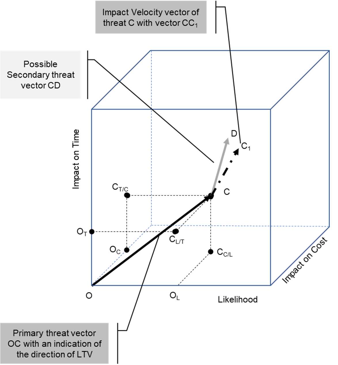
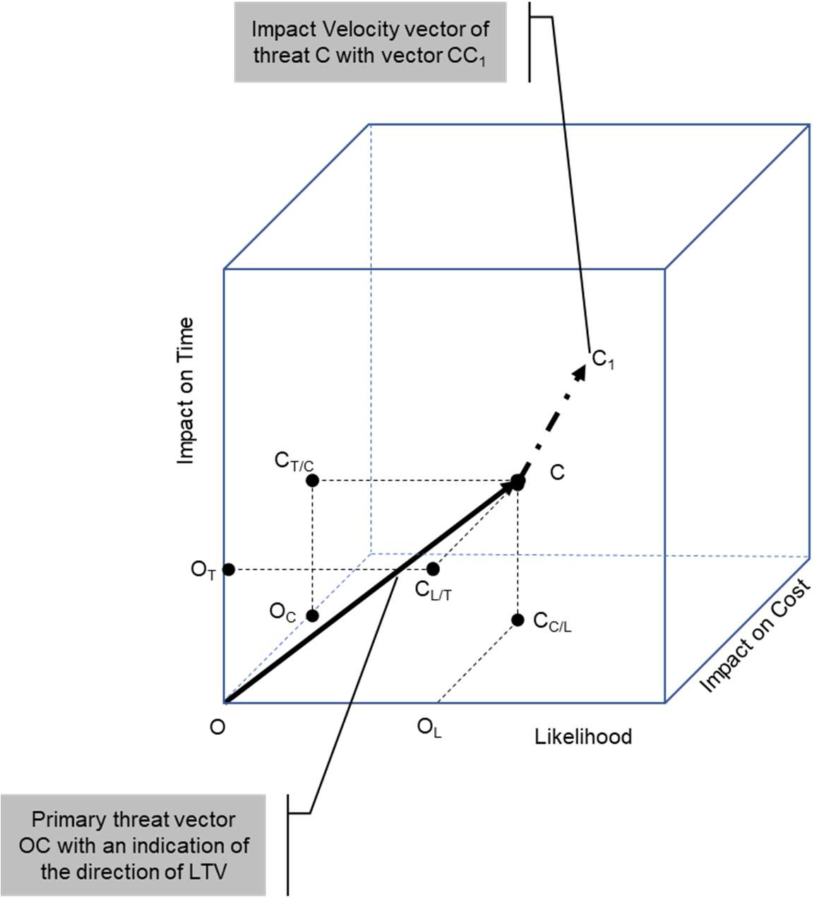
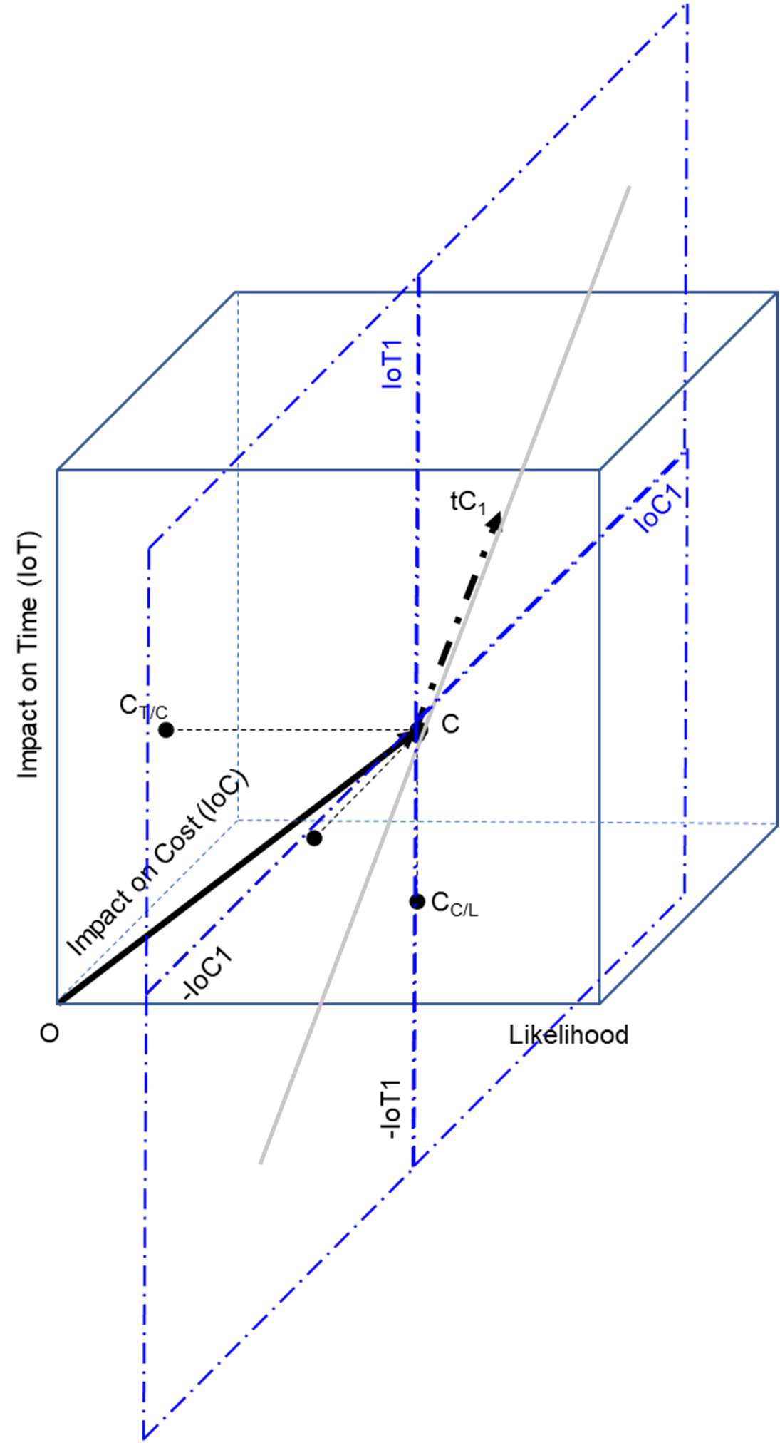
The author, based on the previous analysis done by Antoniadis & Thorpe (2003), proposes that a risk located at coordinates (L, IoT, IoC) within the 3D cube can be represented as a position vector. This vector originates from the point of zero risk, <0, 0, 0>, and terminates at the risk's coordinates. For example, for a risk with L=2, IoT=3 and IoC=3. the risk will terminate at point C and have coordinates <2,3,3>. This primary vector, which we will call OC, represents the path the risk takes as it materialises.
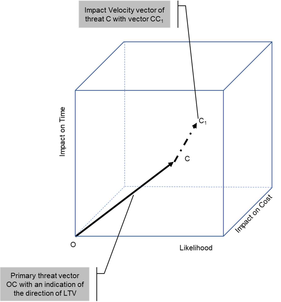
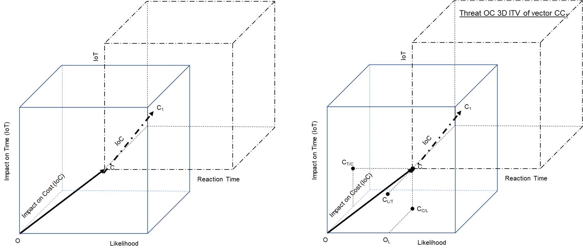
Once the risk occurs at point C, a secondary velocity vector, CC1, can emerge, representing the escalation of its impact over time. This is presented in Figures 4a & 4b below. In addition to vector CC1 and if a secondary threat is to occur, this will be represented by another vector CD.
This shift from a scalar (a simple number, like a product score) to a vector representation has profound implications. A vector inherently contains richer information about the risk it represents:
This vector-based framework provides the necessary mathematical foundation to model Lead Time Velocity (LTV) and Impact Time Velocity (ITV) not as abstract qualitative scores, but as distinct, quantifiable vectors. The primary threat vector OC models the LTV, describing how quickly the risk moves from a state of potential to actual occurrence. Theoretically, this will be moving from the origin with coordinates <0,0,0> to point 'C' with coordinates <1,3,3>. The secondary vector CC1 models the ITV, describing how rapidly the consequences escalate after the event.
To fully unlock the predictive power of this new model, we must first establish the underlying mathematical principles that govern vectors in 3D space. By understanding the vector equation of a line, we can begin to model the trajectory and velocity of risks with unprecedented analytical rigour.
To operationalise the vector-based risk model, a foundational understanding of vector mathematics is essential. This section demystifies the core principles, focusing on the vector equation of a line. This equation, a staple of physics and geometry, becomes a remarkably powerful tool for risk analysis when one of its key parameters is reinterpreted in the context of project management.
The general formula for the vector equation of a line in 3D space is:
→r(t) = →r0 + t →v
Each component of this equation has a specific meaning:
The pivotal argument for applying this to risk management lies in the interpretation of the parameter 't'. In pure mathematics, 't' is merely a scalar. However, in physics/kinematics as also in the context of project management, which operates entirely within the dimension of time, 't' is not just a scalar but should be interpreted as a time variable, measured in units such as hours, days, or weeks.
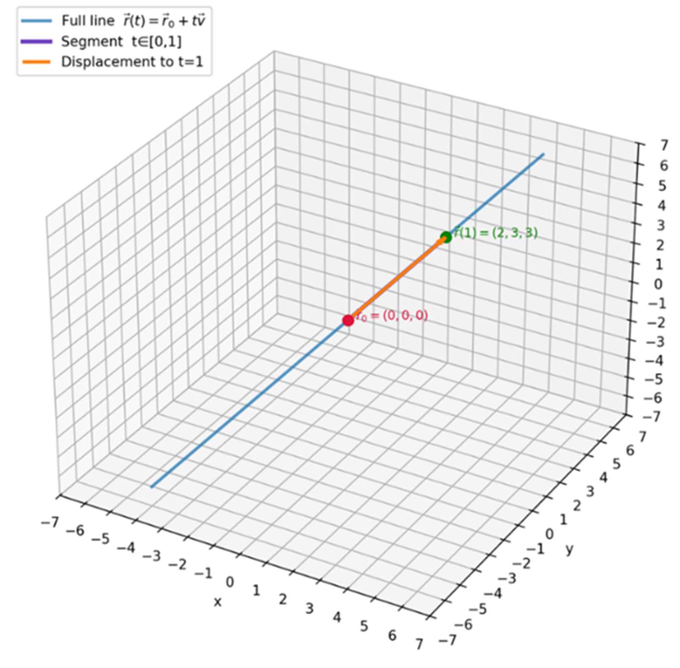
Where traditional risk scores are dimensionless products, the vector equation r(t) = r₀ + t v embeds the risk within the dimension of time, making its growth or decay a measurable function of the project schedule. This interpretation has a critical impact. It transforms the static equation of a line into a dynamic model of movement. For example, consider a risk vector originating from <0, 0, 0> with a direction vector of <2, 3, 3>. Its equation becomes r(t) = <2t, 3t, 3t>. If we allow time t to slip from 1 unit to 2 units, the risk's coordinates double from <2, 3, 3> to <4, 6, 6>. The use of vectors immediately and visually emphasises the escalating effect that the passage of time has on the risk's magnitude.
The figures below (Figures 5a & 5b) visually demonstrate this principle. As time (t) doubles from 1 to 2, the risk's position vector moves from r(1) = <2,3,3> (see Figure 5a) to r(2) = <4,6,6> (see Figure 5b), further from the origin along the same trajectory, graphically representing the increase in its overall magnitude.
Explanation:
Using vector equation →r(t) = →r0 + t →v with r0 coordinates <0,0,0> and introducing coordinates for vector ‘v’ as <2,3,3> Figure 5a presents this in 3D.
The figures below (Figures 5a & 5b) visually demonstrate this principle. As time (t) doubles from 1 to 2, the risk's position vector moves from r(1)=<2,3,3> (see Figure 5a) to r(2)=<4,6,6> (see Figure 5b), further from the origin along the same trajectory, graphically representing the increase in its overall magnitude.
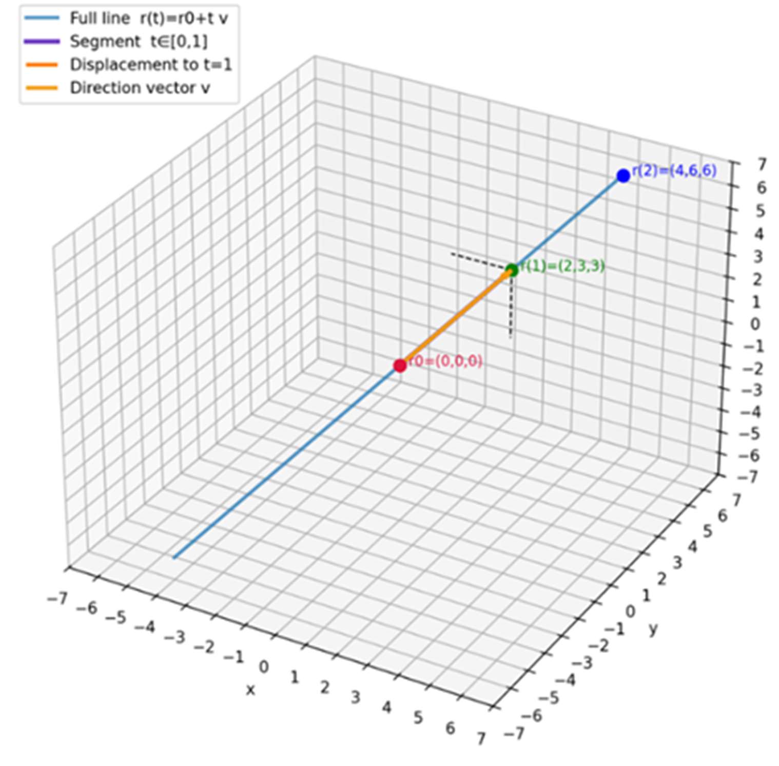
As seen in Figures 5a and 5b, if the initial starting point ro is the origin <0, 0, 0> and the direction vector v <2, 3, 3>, then the position vector 'r' at 't=1' is <2, 3, 3>, but if the time 't' slips to 't=2', the position vector immediately doubles in size to <4, 6, 6>. This clearly shows how the use of vectors emphasises the effect of the time element on the risk (LTV).
With this mathematical framework established, where risks are vectors and the parameter 't' represents time, it is now possible to construct a comprehensive model. This model will define Lead Time Velocity (LTV) and Impact Time Velocity (ITV) as specific, interacting vectors that together describe the full dynamic lifecycle of a risk within the 3D risk space.
This section represents the culmination of the preceding concepts, formally defining a complete, dynamic risk model. This framework is comprised of two key vectors that together capture the temporal journey of a threat: the Lead Time Velocity (LTV) vector, which describes its path to occurrence, and the Impact Time Velocity (ITV) vector, which models the escalation of its consequences.
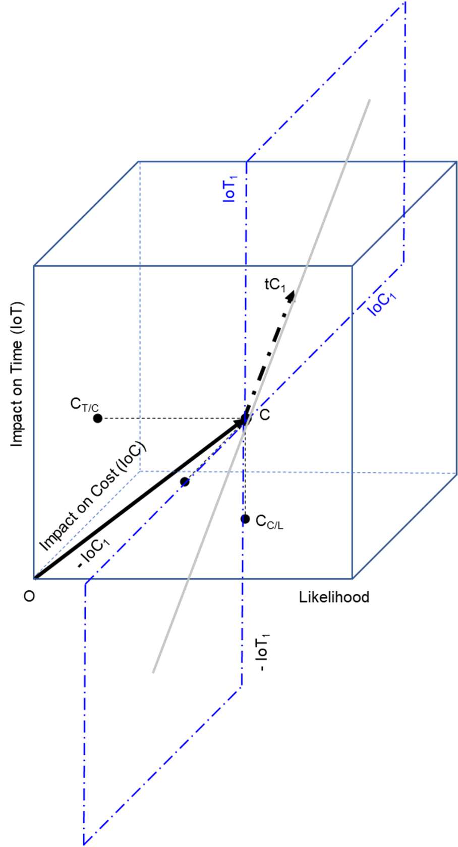
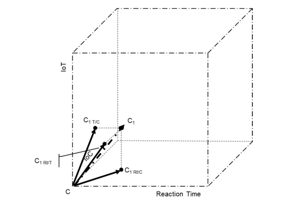
The Lead Time Velocity (LTV) is represented by the primary threat vector OC. This vector originates at the point of zero risk, <0, 0, 0>, and terminates at the coordinates of the identified risk C = (L, IoT, IoC) within the 3D cube. The vector OC embodies the speed and trajectory at which a potential threat approaches its point of materialisation. Its magnitude indicates the overall severity, while its direction reveals the nature of the impending impact, as shown in Figure 6 below, which depicts the primary threat vector OC and the subsequent Impact Time Velocity vector CC1.
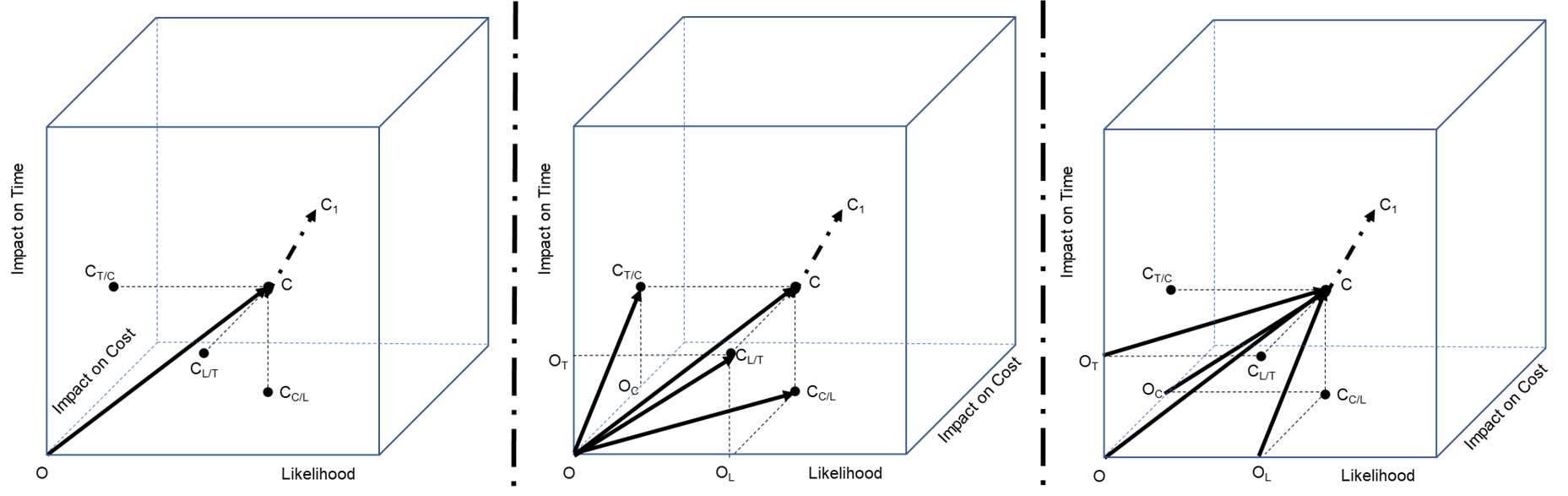
To enable targeted risk management, the LTV vector OC can be deconstructed into its component vectors on the 2D planes defined by the primary axes (see Figure 7a & 7b below). As shown in the figures below, these components isolate the LTV, risk velocity in relation to pairs of variables. For example, the component vector OC_T/C in the plane defined by IoT & IoC, represents the speed of the LTV threat as a combination of its Impact on Time and Impact on Cost elements.
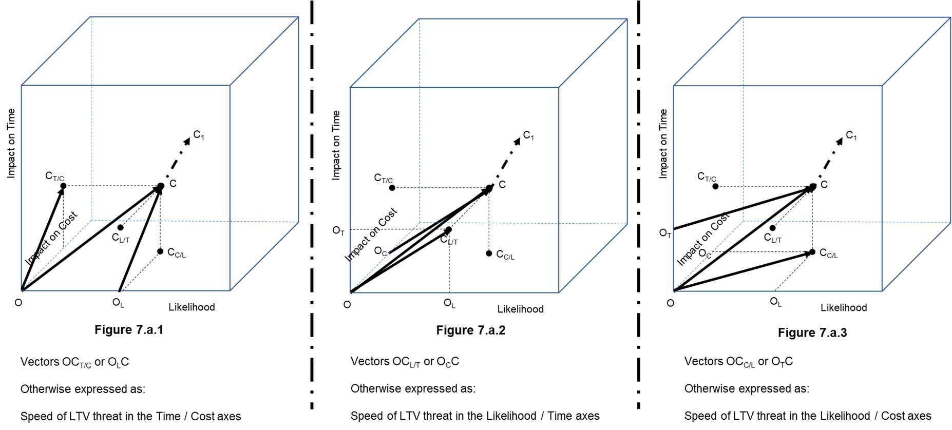
This deconstruction provides a direct link between the vector model and practical risk management actions. This vector-based deconstruction allows, for the first time, a direct mathematical and visual link between specific management actions (controls vs. mitigation) and their intended effect on the threat's trajectory and magnitude. The two distinct strategies for managing risk align perfectly with these vector components:
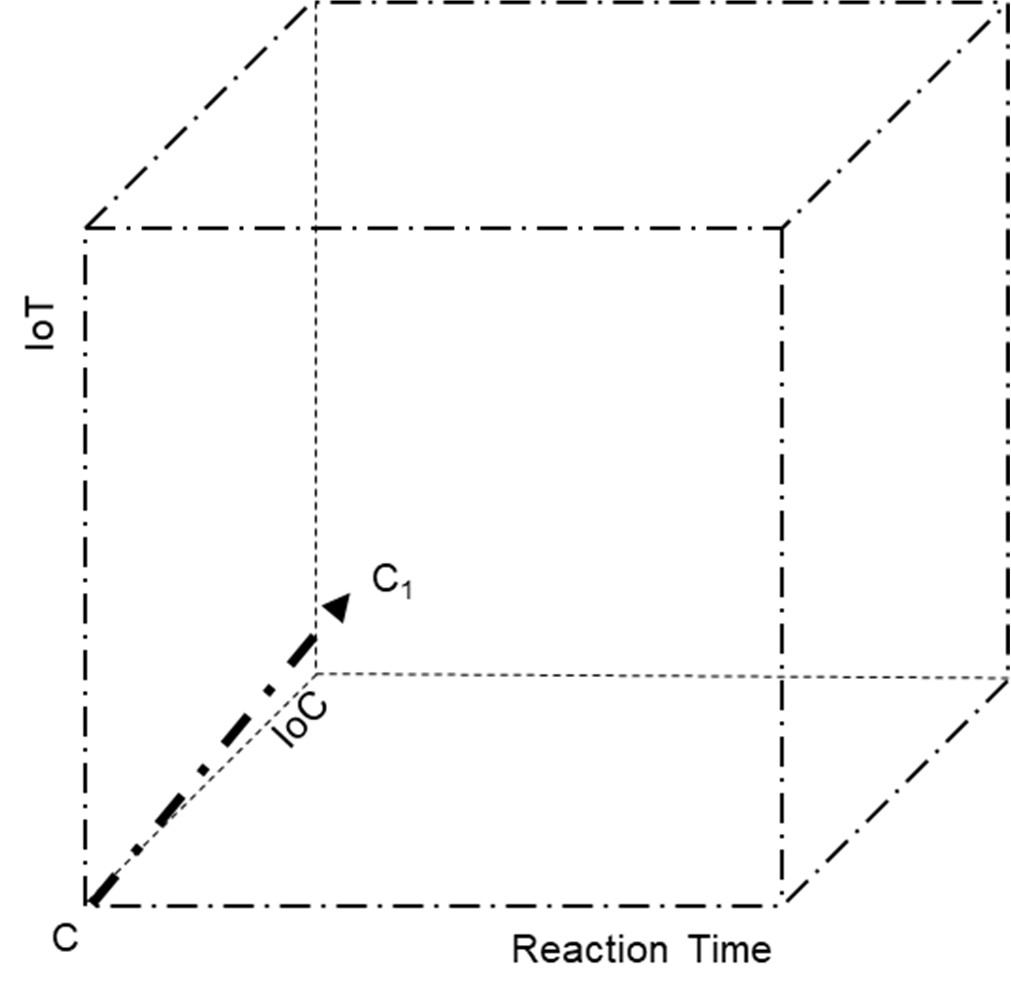
Once a risk event occurs at point C, its likelihood is no longer a variable; it has happened. At this moment, a second velocity becomes critical: the Impact Time Velocity (ITV). The ITV is represented by the secondary vector CC1, whose origin is at point C, the endpoint of the LTV vector. This vector models the rate and direction at which the damage escalates after the initial occurrence.
Two potential models are proposed for how this ITV vector operates:
The 2D plane in which ITV acts can be presented as part of the overall 3D cube and this is shown in Figures 9, 10 & 11 below.
Figures 13 and 14 below present the 3D cube on which the ITV vector CC1 acts, with the relevant axes, see Figure 13 and with its components in Figure 14.
Regardless of the model used (2D or 3D), the total risk at any moment after the event materialises can be expressed by a simple but powerful vector equation. The total risk is the sum of the initial risk vector and the subsequent impact velocity vector scaled by the elapsed time:
Here, OC is the initial risk vector at the moment of occurrence, and 't' is the time that has elapsed since the risk occurred. This simple equation transforms risk assessment from a static exercise into a predictive, time-based model of potential damage escalation, allowing for quantitative analysis of a developing crisis.
The author has attempted to present a fundamental evolution in risk assessment, arguing for a shift from a static, point-based methodology to a dynamic, vector-based model. By incorporating the temporal dimensions of Lead Time Velocity (LTV) and Impact Time Velocity (ITV) into a three-dimensional risk space, organisations can gain unprecedented insight into the true nature of threats. This approach moves beyond simply asking "what is the risk?" to answering the more critical questions of "how fast is it coming?" and "how quickly will the damage escalate?"
The primary advantages of adopting this 3D vector-based methodology are transformative, offering greater clarity, proactivity, and analytical rigour.
The concepts presented here lay the groundwork for significant future development and practical application. Avenues for future work include:
Ultimately, by embracing the mathematics of vectors and the physics of velocity, this methodology has the potential to transform risk management. It can elevate the practice from a reactive, compliance-driven exercise into a truly predictive and strategic discipline, empowering project leaders to navigate uncertainty with greater foresight and confidence.
The author wishes to indicate that Figures 5a & 5b, which present a visualisation of the vectors in 3D were generated using Copilot.
.png)
.png)


